Step 2: Design fair pricing
A practical framework for Responsible AI in algorithmic pricing
How do you build a fair pricing model?
Step 1 established what fairness means for your product and which criterion you are required to meet. Step 2 is about building a model that actually achieves it. That sounds straightforward but involves a decision most modelling teams do not make explicit: at what stage in the pricing pipeline do you enforce fairness?
There are three points at which you can intervene. You can adjust the data before the model sees it (pre-processing). You can build fairness directly into the model’s training objective (in-processing). Or you can adjust the model’s predictions after training is complete (post-processing). Each approach works best for different fairness criteria. The choice should follow from Step 1, not from what is easiest to implement.
Mini-glossary
Notation follows Step 1: Define fairness.
| Symbol | Plain language |
|---|---|
| X_P | Protected attribute (e.g. gender, race, ethnicity) |
| X_{NP} | Non-protected rating features |
| \hat{Y} | Predicted value of the chosen outcome variable. Pure premium by default in this step’s models, per the scope note above |
Model labels follow Xin and Huang (2024).
| Label | Plain language |
|---|---|
| M0 (full model) | Baseline that uses all variables including protected attributes. Kept for comparison, not deployed when discrimination is prohibited |
| MU (unawareness) | Trained without the protected attribute. Targets fairness through unawareness (FTU) |
| MDP (demographic parity) | Fit on debiased non-protected predictors so average predicted outcomes are approximately equal across protected groups |
| MCDP (conditional demographic parity) | Fit on legitimate predictors plus debiased non-legitimate predictors. Group differences are allowed only through legitimate variables |
| MC (CPV) | Full model (M0) fitted, then predictions averaged over protected groups at scoring time |
| Pre-processing | Change inputs before model training (used by MDP and MCDP) |
| In-processing | Enforce fairness constraints during training (e.g. regularisation or penalty terms in the objective) |
| Post-processing | Change outputs after model training (used by MC) |
Model designs
The four designs below (M0, MU, MDP/MCDP, MC) cover the main approaches in the actuarial literature (Xin and Huang 2024). Côté et al. (2025) provide a broader causal taxonomy of fairness methods in insurance, classifying approaches as best-estimate, unaware, aware, hyperaware, or corrective, which can help map additional methods to the criteria in Step 1. Charpentier (2024) provides a book-length treatment of discrimination, bias, and fairness methods in insurance, including technical tools for quantifying and mitigating discrimination.
M0: The baseline
Before building any fair model, fit a baseline that uses all available variables including the protected attribute. This is M0. You will not deploy M0 in a market where discrimination is prohibited, but you need it for two reasons. First, it gives you the best available estimate of the true expected cost for each group, which you need for welfare analysis in Step 3. Second, it provides the benchmark against which to measure how much fairness constraints affect accuracy and pricing.
MU: Removing the protected attribute
The simplest approach is to remove the protected attribute from the training data and fit the model on everything else. This is what most insurers already do, either because they do not collect the protected variable or because regulation prohibits its use.
The limitation is real and important. Removing a variable does not remove its influence when other variables in the model are correlated with it. If postcode is correlated with race, and race is the protected attribute, then a model using postcode will still partially reflect race in its outputs. MU prevents direct discrimination but does nothing about indirect discrimination through proxy variables. It is a necessary starting point, not a sufficient solution for jurisdictions concerned with proxy effects.
MCDP: Separating legitimate from non-legitimate variation
MCDP suits situations where some price differences between groups are legally justified and some are not. A risk-rated insurer will charge higher premiums to customers with more claims history. If those customers happen to be disproportionately from a protected group, that price difference is defensible as long as claims history is accepted as a legitimate factor by the regulator. What is not defensible is a price difference that arises because other variables in the model are acting as proxies for the protected attribute.
The model works in two stages. First, legitimate predictors (those the regulator accepts as grounds for price variation, such as claims history, vehicle type, or annual mileage) are kept in the model unchanged. Second, other predictors are stripped of their correlation with the protected attribute before the model is fitted. One approach is orthogonalisation (Kamiran and Calders 2012); another is optimal transport, which remaps the distribution of each predictor to remove its dependence on the protected attribute (Lindholm et al. 2024b). A variable that was correlated with race or gender is adjusted so that its value no longer carries that information. Once this pre-processing is complete, the model is trained on the adjusted dataset. The result is a model where price differences between groups can only arise through the legitimate variables.
This is the model design that best maps to conditional demographic parity (CDP), which is the criterion most directly relevant to regulatory proposals in Colorado and New York. Case Study: Fair Models works through a full implementation.
MDP: Demographic parity across all variables
MDP is a stricter version that does not distinguish between legitimate and non-legitimate predictors. All non-protected predictors are debiased before the model is fitted, so that average predicted outcomes are approximately equal across protected groups unconditionally.
This is appropriate for regulatory environments that require demographic parity rather than conditional demographic parity: for example, where the regulator expects equal average premiums across groups regardless of whether legitimate factors explain the difference. It involves a greater sacrifice of actuarial accuracy than MCDP because it removes the group-predicting power of all variables, including legitimate ones. In markets where fine risk classification is commercially important, this trade-off deserves explicit consideration.
MC: Averaging over the protected attribute
MC takes a conceptually different approach. Instead of changing the data before training, it changes how predictions are used. A full model (M0) is fitted that includes the protected attribute, giving the best actuarial estimate of expected cost for each combination of characteristics. At the point of scoring, rather than using M0’s prediction directly, the model computes a weighted average of M0’s predictions across all protected-group values. Each customer receives a price that reflects their non-protected characteristics but does not depend on which group they belong to.
In practice, the model takes the full-information prediction and averages it across all possible values of the protected attribute, keeping everything else about the customer unchanged. The result is a price that reflects the customer’s non-protected characteristics but does not depend on which group they belong to. For technical readers, the formula is:
\hat{Y}_{MC} = \frac{1}{N}\sum_{j=1}^N \hat{f}_{M0}(X_{NP}, X_P = x_{p_j})
The advantage is better predictive accuracy: MC uses all available information in estimating expected costs. The price each customer sees does not directly use their protected group membership, but the model’s internal estimates do. This approach was introduced as the discrimination-free price by Lindholm et al. (2022) and implemented in the insurance context by Xin and Huang (2024). It targets the fairness criterion of controlling for the protected variable (CPV).
Causal approaches
The model designs above treat fairness as a statistical property of inputs or outputs. A causal approach goes further, asking which pathways from rating variables to prices are permissible. If a variable influences price partly through a protected attribute (for example, postcode partly proxies race), a causal model can block that specific pathway while preserving the legitimate influence of the variable. This requires specifying a causal graph: a diagram of which variables cause which outcomes and through which routes.
Araiza Iturria et al. (2024) derive a discrimination-free premium explicitly under a causal framework in the insurance context, extending the statistical approach of Lindholm et al. (2022). Côté et al. (2025) implement a broader causal taxonomy of fairness methods in insurance, classifying approaches as best-estimate, unaware, aware, hyperaware, or corrective depending on how much causal information is incorporated. Causal methods are more demanding to implement (they require domain knowledge about causal structure in addition to data) but more precise about what discrimination they remove.
Matching model to criterion
| Model | Criterion | Approach |
|---|---|---|
| M0 (full) | Baseline | Uses X_P and X_{NP} |
| MU | FTU | \hat{Y} = f(X_{NP}) only |
| MDP | DP | Pre-process all X_{NP} to X_{NP}^{\star} |
| MCDP | CDP | Retain legitimate predictors; debias non-legitimate predictors |
| MC | CPV | Fit M0; average over X_P at prediction |
How regulation maps to model design
Xin and Huang (2024) maps regulatory regimes to fairness criteria and standard model designs.
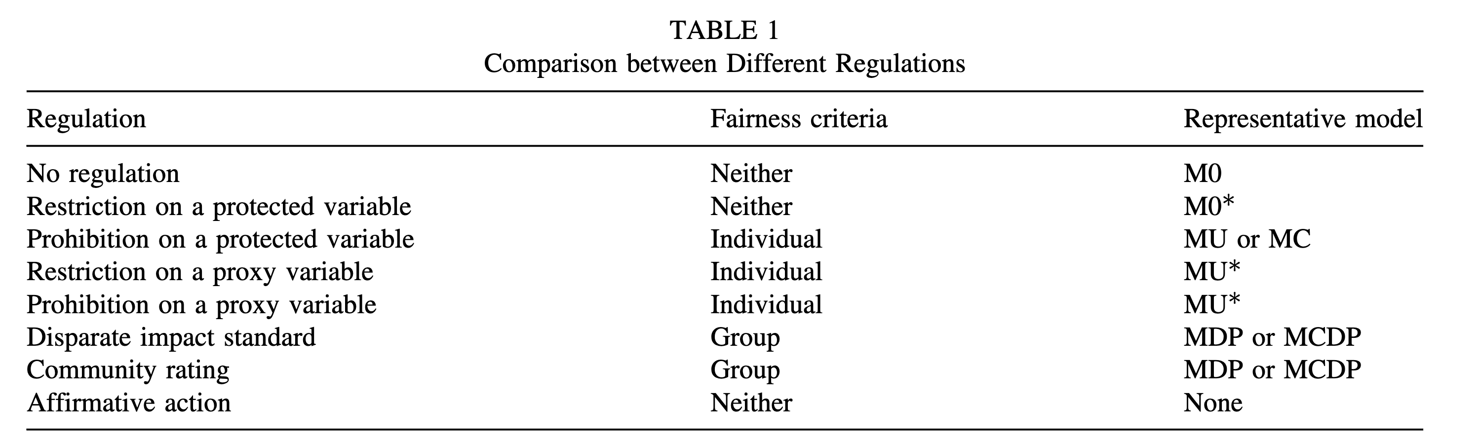
The progression from left to right in the diagram is a progression in how much cross-subsidy regulation requires. At the left extreme, no regulation: the insurer can use any variable and individual actuarial pricing prevails. At the right extreme, community rating: everyone pays the same premium and cross-subsidy is complete. Most markets sit somewhere in the middle, and the right model depends on where.
Pre-processing
Pre-processing enforces fairness by adjusting the input data before the model is trained. The idea is to remove or reduce the correlation between non-protected variables and the protected attribute, so that the trained model cannot learn to proxy the protected group from the adjusted inputs.
MDP and MCDP both use pre-processing. In MDP, all non-protected predictors are debiased unconditionally. In MCDP, only non-legitimate predictors are adjusted while legitimate predictors are kept unchanged. Techniques include orthogonalisation (Kamiran and Calders 2012) and optimal transport (Lindholm et al. 2024b). Pre-processing is applied once before training and does not require changes to the model architecture or training procedure, making it relatively easy to slot into an existing modelling pipeline.
In-processing
In-processing builds fairness into the model training step rather than adjusting inputs or outputs. One approach adds a penalty to the model’s training objective, a cost that increases whenever the model violates the chosen fairness criterion. The model then learns to balance predictive accuracy against fairness, with a single parameter controlling how much weight to give each goal.
In-processing is particularly useful in price optimisation, where the optimiser’s goal (typically maximising expected profit) can be extended to include a fairness constraint. Case Study: Welfare Implications implements this in the pricing-rule context (PDP and PAF rules in Step 3). A multi-task neural network approach embeds the fairness criterion directly into training, with the advantage that the protected attribute is not required at prediction time (Lindholm et al. 2024a).
Post-processing
Post-processing enforces fairness by adjusting the model’s predictions after training is complete. The underlying model is fitted without fairness constraints, giving the best available estimate of expected cost. At the point of scoring, predictions are modified to meet the fairness criterion.
MC is the post-processing design in this playbook. It takes the full-model predictions and averages them across all values of the protected attribute for each customer. The customer receives that average as their price rather than the group-specific prediction. Post-processing leaves the model itself unchanged and is therefore straightforward to apply to an existing production model, though it requires the protected attribute to remain available at scoring time for the averaging step (Lindholm et al. 2022; Xin and Huang 2024).
The fairness–accuracy trade-off
A common concern when fairness constraints are proposed is that they will make the model substantially less accurate, leading to adverse selection and commercial harm. The evidence from Xin and Huang (2024) on a standard French motor insurance dataset is more reassuring than the concern suggests.
Fair models including MCDP and MC achieved loss ratios (claims paid as a share of premiums earned) close to those of the unconstrained M0 baseline. The reduction in predictive accuracy was modest while the reduction in premium disparities between protected groups was substantial. Fairness-constrained XGBoost models retained most of their predictive edge over GLMs while also meeting fairness criteria that GLMs alone might not satisfy.
This does not mean the trade-off is zero. An insurer that enforces strict demographic parity will accept greater exposure to adverse selection (the tendency for lower-risk customers to leave the pool when they are cross-subsidising higher-risk customers, leaving a less profitable book), because it will price some high-risk customers identically to lower-risk customers in the same protected group. The relevant question is whether the magnitude of that exposure is acceptable given regulatory requirements and competitive pressures. That is a business decision, but it can be quantified, and the numbers in this context are smaller than critics of fairness regulation often assume.
Addressing indirect discrimination through proxy removal (MCDP) also produces a side benefit: because the model cannot use proxies for the protected attribute, it reduces the risk that the fair model inadvertently attracts a systematically different risk pool. The adverse selection concern associated with fairness constraints is partly offset by the reduction in proxy variables within the model.
Implementation
- Link each model (M0, MU, MDP, MCDP, MC) to the criterion chosen in Step 1
- Retain baseline M0 for welfare and audit comparisons in Steps 3 and 4
- Document the pre-processing, in-processing, or post-processing choice and produce a reproducible pipeline
- Agree the list of legitimate vs non-legitimate variables with legal and compliance before modelling begins
Checklist
Use this checklist to confirm model design choices before welfare analysis. Assign an owner for each item and record sign-off.
| Task | Typical owner |
|---|---|
| Model (M0, MU, MDP, MCDP, MC) linked to Step 1 criterion | Actuarial and data science |
| Legitimate vs non-legitimate variables listed and signed off | Legal and compliance, actuarial |
| Baseline M0 retained for downstream comparisons | Model risk |
| Versioned data, code, and parameters | Data science and MLOps |